Summer Goals, starting a blog in an hour a day, and Iris

April 30, 2018 in DATA SCIENCE
data exploration
5 minute read

Being in school is great—at the end of each semester, I feel like I can restart my life and make New Year’s Resolutions. My big resolution now that winter semester is over is to develop a data science portfolio in the form of a blog.

I can’t dedicate my whole summer to blogging, but I am pretty confident that I can carve out an hour of time every day to spend on this. My plan is to use the following schedule each week and crank out a post each Friday.

Monday:

Define the project scope: write 5-7 questions (30 min)
Study practical / business importance, write intro (25 min)
Create Rmd w/ setup, intro, & questions (5 min)

Tuesday:

Get all the data (60 min)
- Write out required data points (10 min)
- Locate data sources & redefine scope if needed (15 min)
- Collect & tidy the data (35 min)

Wednesday:

Answer questions 1-4 (15 min each)

Thursday:

Answer questions 5-7 (20 min each)

Friday:

Write conclusion (20 min)
Add memes / interesting pictures (15 min)
Review the blog draft, rewrite / finish writing (15 min)
Publish it & advertise on Twitter (10 min)

This post is a test run. I’m going to do a data science 🔬 blog entry in 30 minutes. 30 minutes for two reasons:

30 is a nice tenth of 300 minutes (5 hours).
I just took some Benadryl to medicate some seasonal allergies, and I’m planning to be out cold in about 30.

Here goes!

Monday

Questions

Which feature in the Iris dataset explains the difference in species the best?
I remember that two of the species are a little more similar than the third—is there some biological reason for that?
Does the ordering of the irises in the dataset have any relationship with the data?

Intro

The Iris dataset is probably the first thing I came across when I became interested in machine learning. A biostatistician named Ronald Fisher collected several measurements for three types of irises, Iris versicolor, setosa, and virginica:

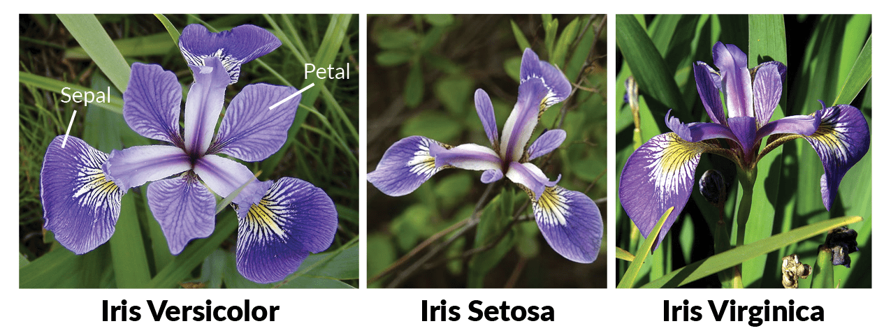
Source: http://www.lac.inpe.br/~rafael.santos/Docs/R/CAP394/WholeStory-Iris.html

Fun fact: my dad is an avid gardener and has about 15 different varieties (species? they’re at least different colors) of iris in his garden in front of my family’s home.

Tuesday

The data I need:

The Iris dataset (built in to R)
Some additional info re: relatedness of iris species (Wikipedia?)

We’ll see if we have time for that additional info.

iris <- as_tibble(iris) %>% 
  rename(
    sepal_length=Sepal.Length,
    sepal_width=Sepal.Width,
    petal_length=Petal.Length,
    petal_width=Petal.Width,
    species=Species
    )
iris %>% head()

## # A tibble: 6 x 5
##   sepal_length sepal_width petal_length petal_width species
##          <dbl>       <dbl>        <dbl>       <dbl> <fct>  
## 1         5.10        3.50         1.40       0.200 setosa 
## 2         4.90        3.00         1.40       0.200 setosa 
## 3         4.70        3.20         1.30       0.200 setosa 
## 4         4.60        3.10         1.50       0.200 setosa 
## 5         5.00        3.60         1.40       0.200 setosa 
## 6         5.40        3.90         1.70       0.400 setosa

Wednesday

Let’s try to tackle the first 2 questions.

Which feature explains the most cross-species variation?

First off, which feature has the most overall variation?

iris %>% 
  select(-species) %>% 
  gather(feature, value) %>% 
  ggplot(aes(x=feature, y=value)) + geom_boxplot()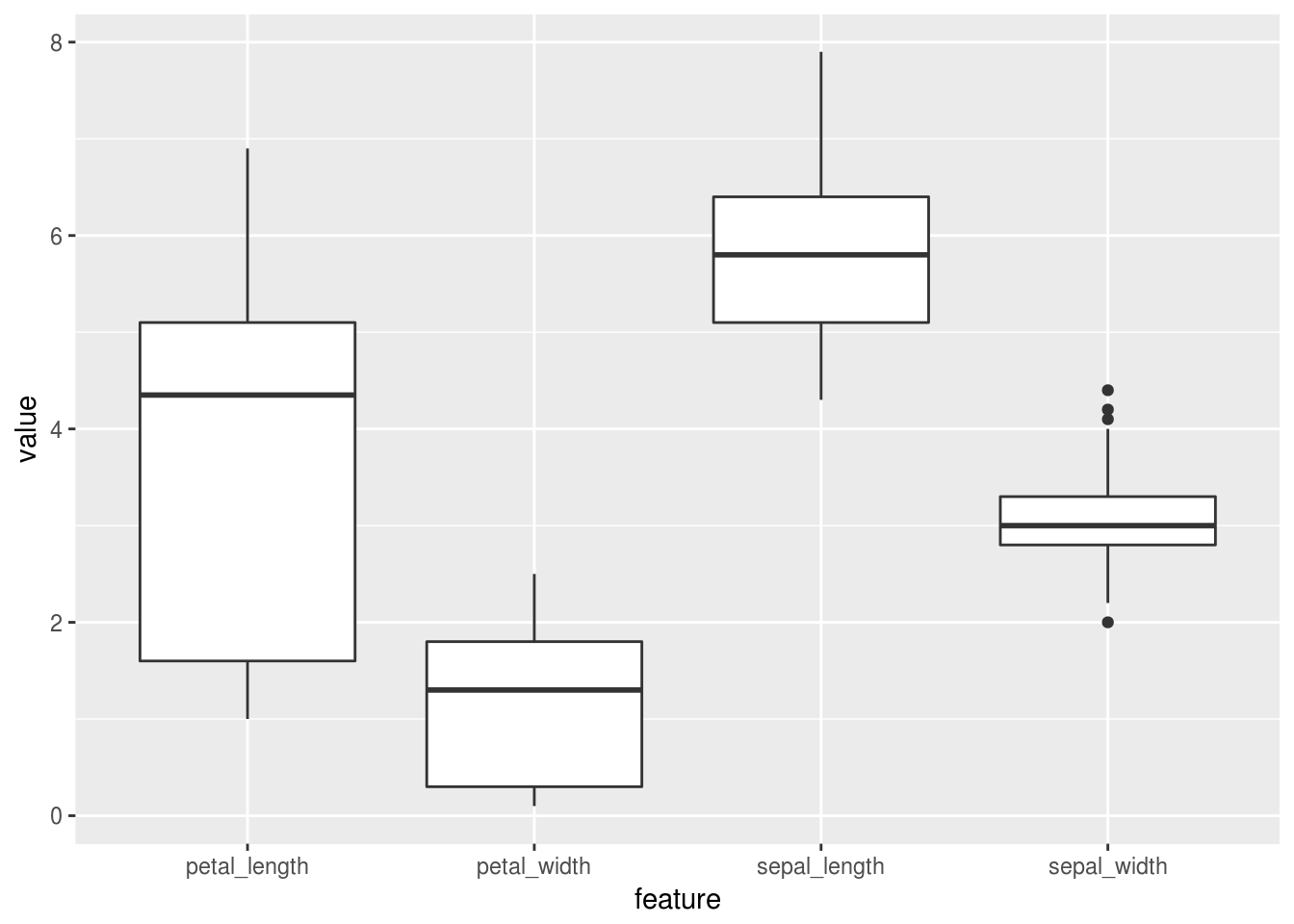

Looks like petal length has the biggest spread of the four features! And it looks like I’m out of time…

Thursday

Does the ordering of the irises relate to the values collected?

In the interest of time, let’s just look at the petal length feature:

iris %>%
  mutate(row_number=row_number()) %>%
  ggplot(aes(x=row_number, y=petal_length, color=species)) + 
    geom_point() + 
    geom_smooth(method="lm")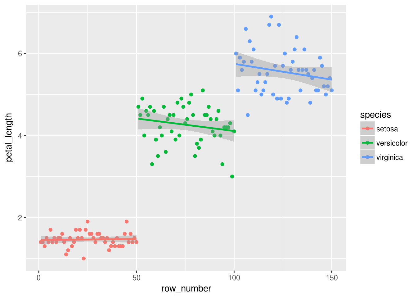

Well, a few things stand out to me:

The setosa clearly have the shortest petals, and the setosa petal lengths seem to cluster more tightly than the other two species.
Both the versicolor and virginica data seem to show a negative relationship between row number. It would be interesting to see if that relationship is:
- From the original dataset (is this the order in which Fisher collected the data? If so, maybe he started underestimating or rounding down the petal lengths as time went on).
- Statistically significant. A good data scientist would take a look at that. But…I’m about out of time!

Friday

We just barely started to get a taste of Iris. Some observations:

The features vary in center and spread. The center thing is pretty obvious—those sepals and petals look a lot longer than they are wide. The spread thing is marginally more interesting. In biology, when a feature is really similar across all members of a species, that’s a hint that that feature may have been selected for. Are bees (or whatever pollinate irises) only attracted to flowers with a certain sepal width? Is there another functional purpose to the widths?
There may be some confounding across row number in the dataset. Well, obviously there is; species are all grouped together. But within each species, there may be some additional confounding.

These are both sorta insignificant observations. But if we were now to do machine learning on this dataset, each observation gives us a little bit of information that can inform our approach. Since the different variables have different centers and spreads in vector space, we would need to normalize before using a distance-based classifier. And if we were fitting a neural net on this data, we would probably want to randomly shuffle the data before training.

The end

I went about 5 minutes over my allotted time. Sixty minutes five times a week will be a rush to make interesting, useful blog entries, but I think it will be a fun summer project!

That Benadryl is definitely in my system. Thanks for reading! See you again on Friday!

Data Science, et al.